Maximizing Robotics Performance: Task Scheduling Techniques, Modeling, and Efficient Resource Management

By: Neil Foxman, Senior Systems Engineer, San Diego office

---

How many times have you asked yourself, “There must be an easier way”? When confronted with mundane or repetitive tasks, our inner engineer will naturally look for ways to speed things up or improve our output. But often there are so many variables, it is hard to know how to speed things up. For example, anyone who has prepared mashed potatoes for a large family dinner has encountered this type of problem: Do I cut all the potatoes at once or cut them in batches? What else should I do while some potatoes are boiling? How many pots do I need? How do I do this process more quickly?

This same question applies when designing a robotic system to do a task; the designer must strike a balance between accomplishing a goal within a set amount of time and reducing the number of features that need to be designed. This paper will attempt to break down this universal problem into a model that one can use to better conceptualize the factors at play. Once we have a common toolkit to describe these types of problems, we can then evaluate the total time it would take to complete a task given different parameters. Also, we will discuss higher level phenomena such as the total task duration’s sensitivity to the internal operations, methods to further reduce total task time, and other special cases.

Notably, this paper will focus on how to model a task given a small set of information and generate a heuristic (total estimated task duration). It will not attempt to optimize all the design parameters simultaneously. Using the mashed potatoes example, if I can only choose between using one or two pots to boil the potatoes, it would not be helpful to know that the optimum is 10 pots or 1.5 pots. Instead, the approach presented in this paper assumes we will be knowledgeable of our design space (such as number of pots) and use this information to generate a schedule which can be iterated over for different design parameters using various numerical tools such as MATLAB or Python.

Task Modeling

Model Basics

In this section, we will discover a method of modeling and visualizing a schedule with sequential steps. The goal is to gain familiarity with the proposed model so we can begin to describe more complex cases in later sections.

This model is most useful when a collection of many discrete items needs to undergo many operations. To more formally define what an “item” is, we will only be considering a homogeneous set of items that will all undergo the same process; there should be no branching or sorting items during the task. Next, we define an operation as an activity applied to one or more items that has an associated duration.

We will start with visualizing individual operations and zoom further and further out to gain a larger system-level understanding of the schedule. Let’s assume we are making a robot that helps us make mashed potatoes.

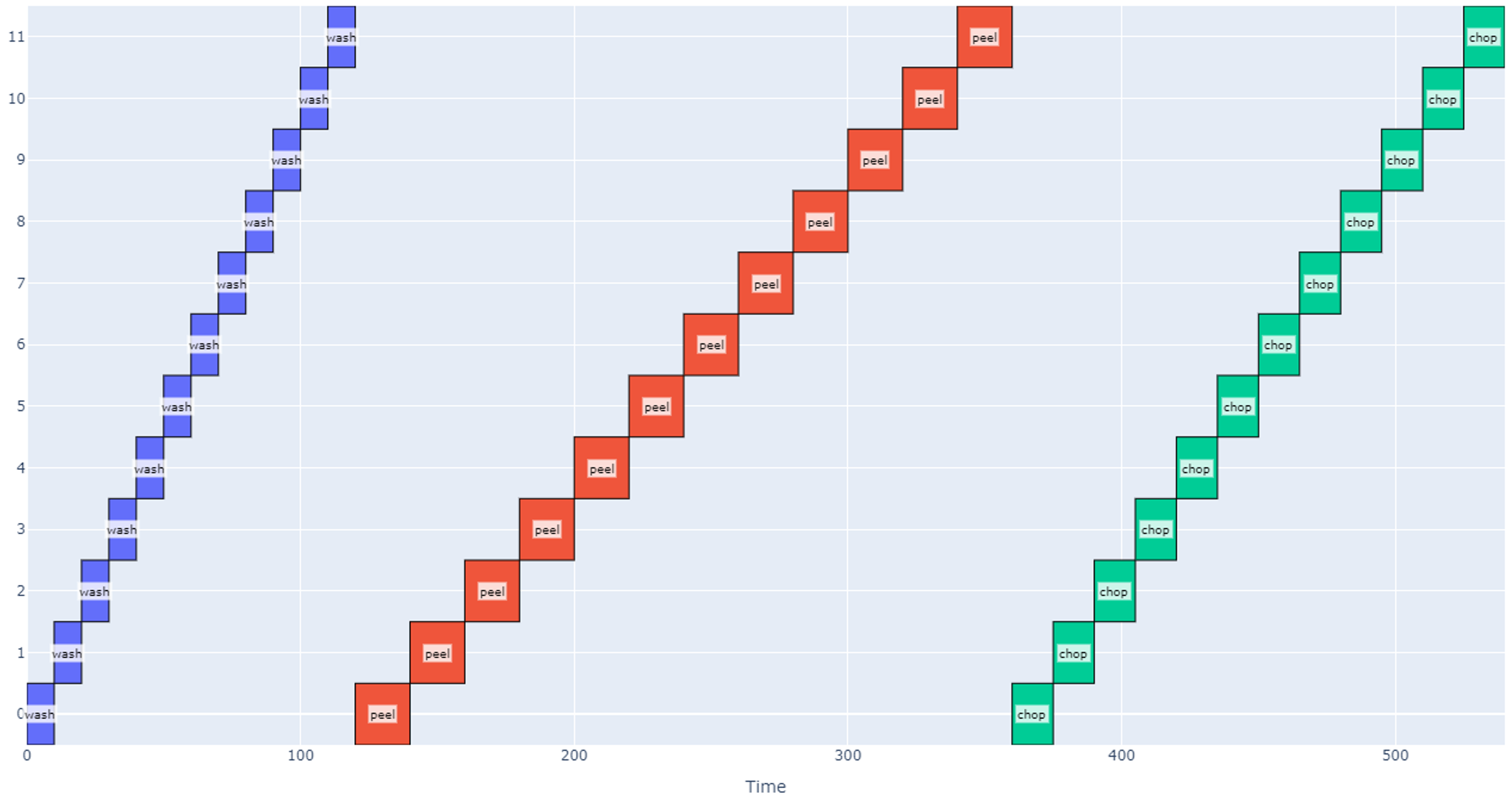
1. The first operation would be to wash the potatoes in a bowl which we can assume takes 10 seconds per potato.
2. Next, the robot would peel each potato which takes 20 seconds per potato.
3. Finally, the robot chops each potato which takes another 15 seconds per potato.

A schedule that accomplishes each of these operations with 12 potatoes is modeled below.

Each item is assigned an index on the vertical axis, and time is represented on the horizontal axis. Each “block” on the graph corresponds to the start and end times for when an operation is applied to a particular item. The total schedule in this case takes 540 seconds (about 9 minutes).

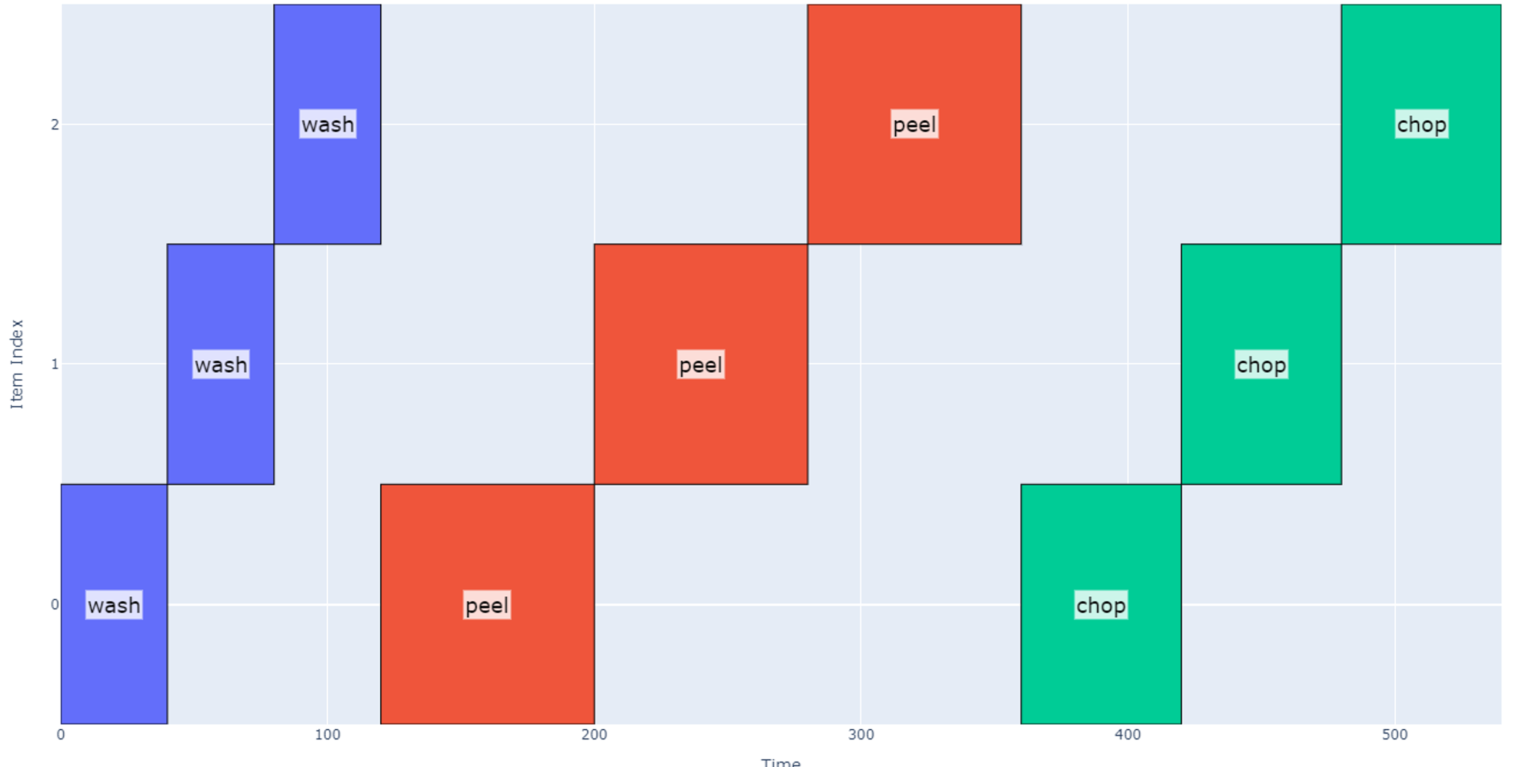
Operations may be hierarchical i.e. each operation can be applied to a group of items. Now let’s represent the case when we operate on the potatoes in groups of four.

1. The first operation would be to wash the four potatoes in a bowl which we can assume takes 40 seconds per group.
2. Next, the robot would peel in groups of four potatoes which takes 80 seconds per group.
3. Finally, the robot chops each potato which takes another 60 seconds per group.

Note that in this case the “item” index (vertical axis) now represents each group of four potatoes instead of individual potatoes to generate a more “zoomed out” view. So far, the total schedule duration is the same, 540 seconds.

Resource Conflicts

This model becomes more interesting when we begin to introduce resource conflicts. A resource conflict is a relationship between operations in a task such that they cannot operate at the same time on different items. We have already seen the common case where an operation has a resource conflict with itself: we have assumed that in the robotic system, we can only cut one potato at a time. Due to the number of moving parts or design complexity, different operations may have a resource constraint on each other.

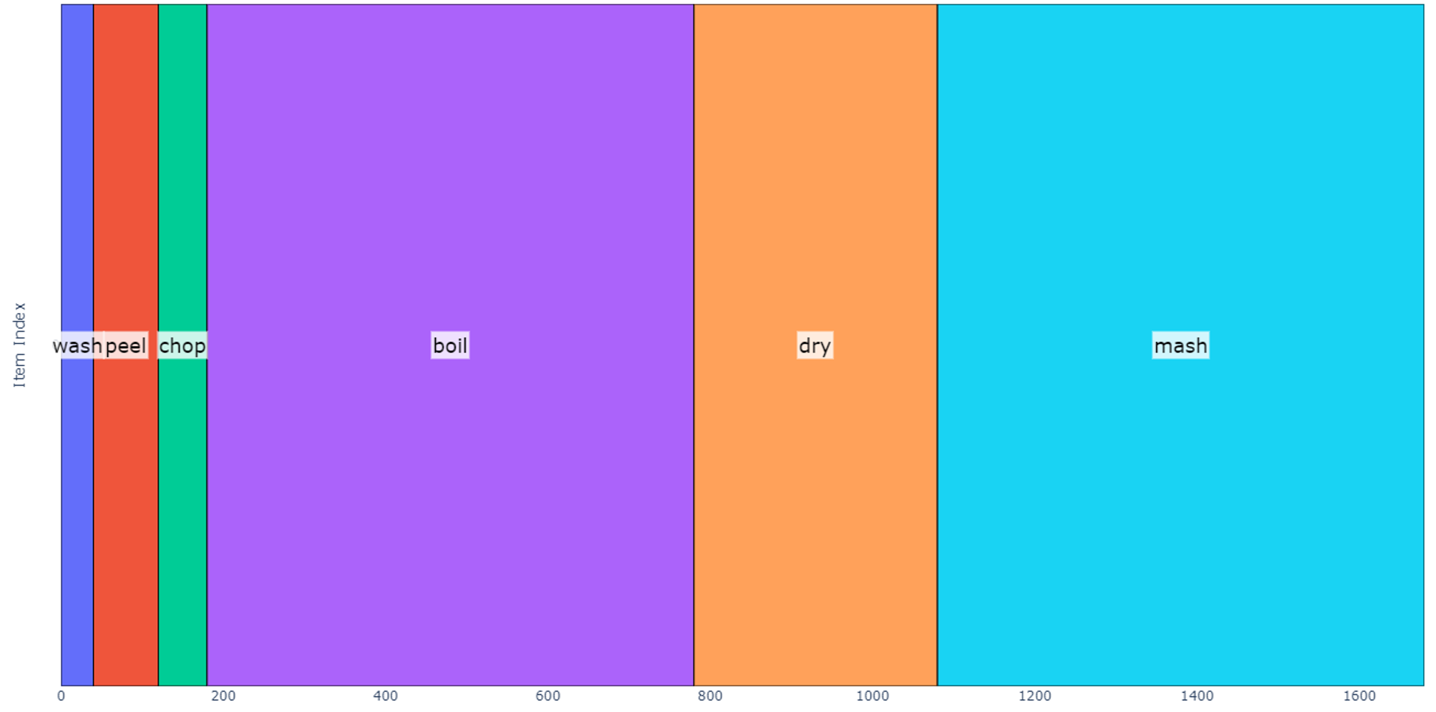
Let us now define an operation sequence as a list of operations that need to be applied to each item. When going through the operation sequence, no operation is started until its predecessor is complete. Making mashed potatoes for a single group of four potatoes could be described as shown below.

1. Wash: 40 seconds
2. Peel: 80 seconds
3. Chop: 1 minute
4. Boil: 10 minutes
5. Dry: 5 minutes
6. Mash: 10 minutes

To simplify our discussion, we will not consider toppings, each operation is a fixed duration, and a single bowl is used to boil, dry, and mash the potatoes. A schedule modeling this operation sequence on only one group of four potatoes is shown below.

The total predicted duration for this schedule is 28 minutes.

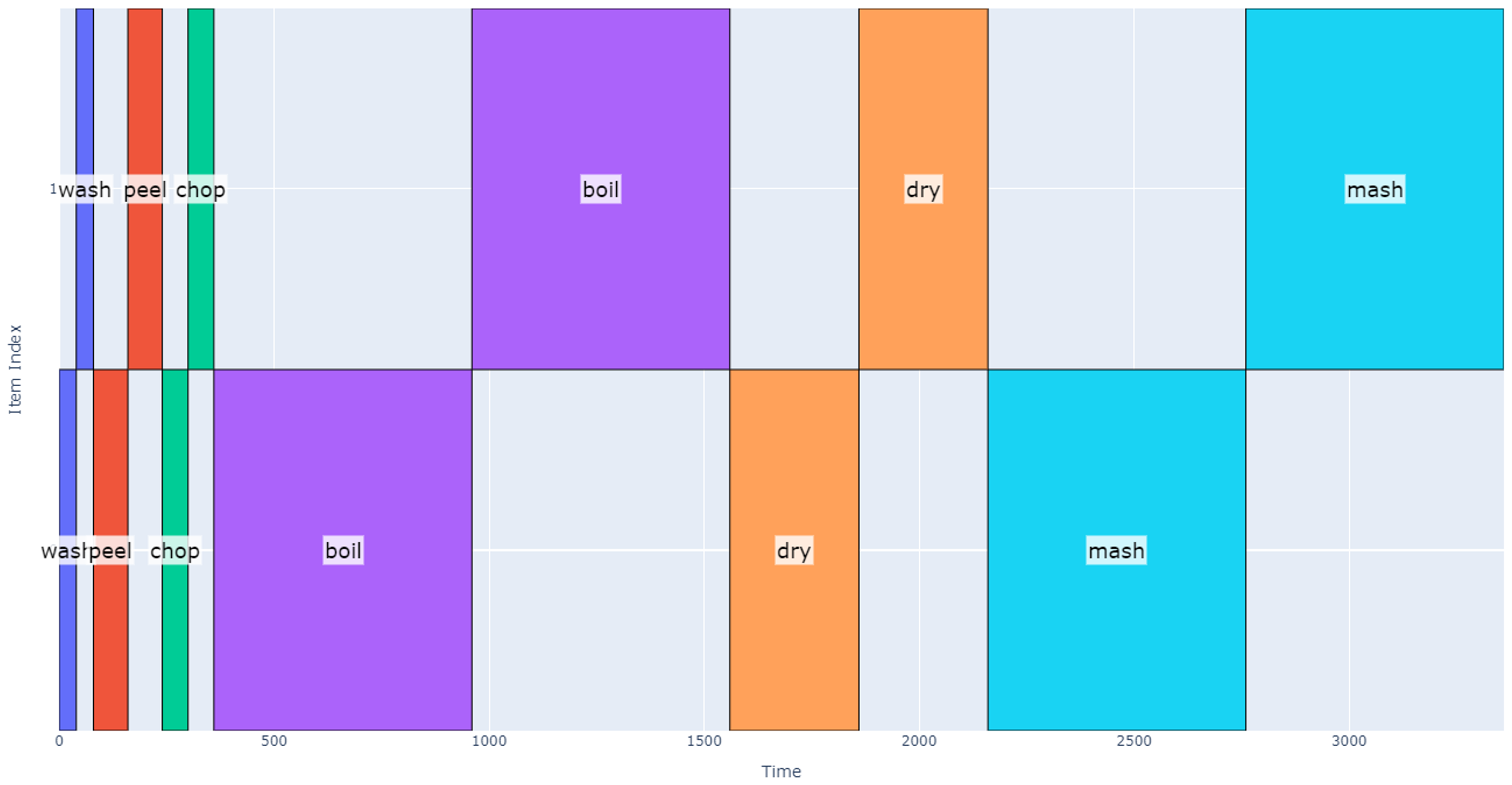
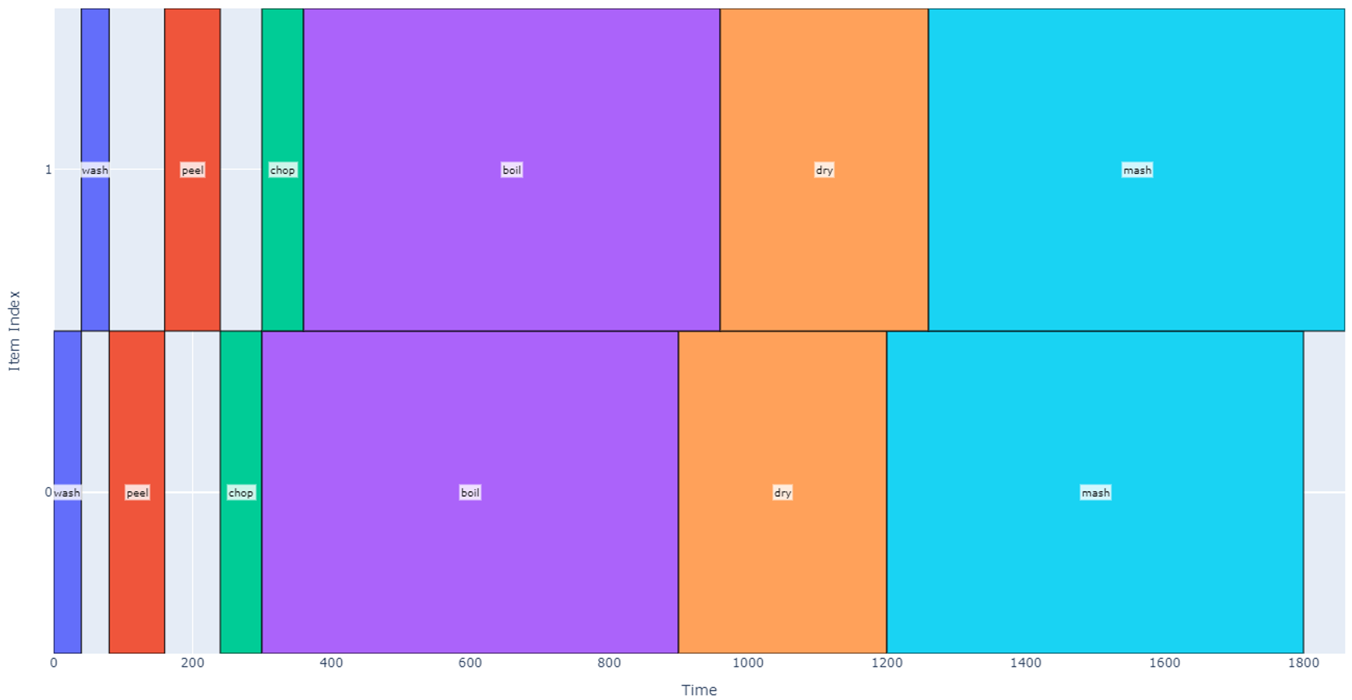
Now we want to scale our operation up to eight potatoes (two groups). We could do this by trivially multiplying the total schedule duration by 2 assuming we start making mashed potatoes with the second group after the first group is complete (total of 28*2=56 minutes). Alternatively, we could wash both groups, then peel both groups, etc. This latter schedule is shown below, but still achieves a total schedule duration of 56 minutes.

The astute observer may find it silly to start the drying process once both groups have completed boiling, but we have assumed there is a resource conflict between the boiling and drying operations. We can optimize our schedule if we better define resource conflicts between operations. Up until now we have assumed that only one operation can be done at a time and that resource conflicts exist between all operations. If we now loosen this restriction, say by using two pots to do the boiling, drying, and mashing, those operations can now occur at the same time. Let’s additionally assume that boiling and drying can occur while we are washing, cutting, or peeling any other group. The resulting schedule is represented below.

Note that after adding a second pot, we have a notable schedule duration reduction, and the total time is now 31 minutes (45% reduction).

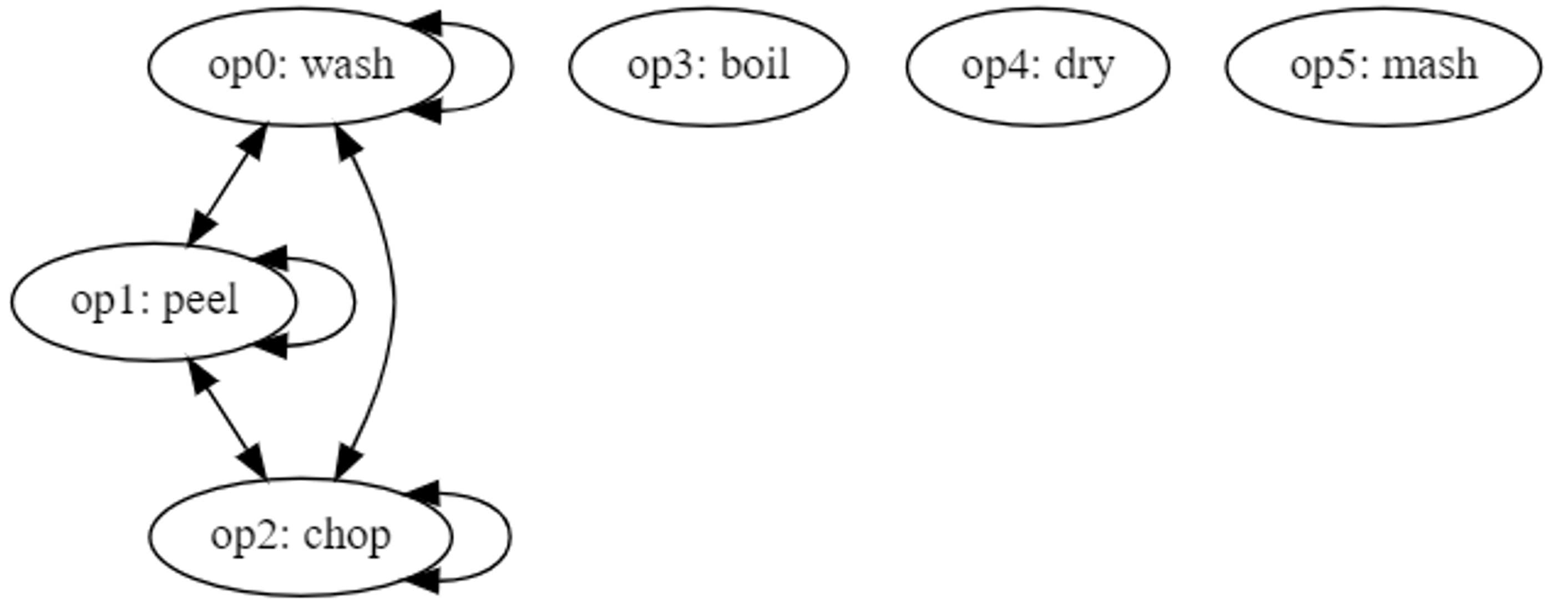
The resource conflicts may be represented using the graph in Figure 1 where each edge represents the relation “has a resource conflict with.”

Figure 1

Conflicts may then be represented programmatically in a scheduling algorithm using an adjacency matrix.

In the example above and for the remainder of this paper, we will assume that all conflicts and all edges are bidirectional for simplicity: neither operation can be started if the other is running.  However, one could imagine a more advanced conflict graph that uses only single-direction edges.  In this case, each edge would signify that operation A “cannot be started while” operation B is running, but operation B may be started while operation A is running. One could add further detail to the conflict graph by assigning weights to each edge.  Weights would allow one to assign a maximum number of operations to be run in parallel until a conflict occurs. Each of these extensions of the conflict graph would also require updates to the scheduling algorithm, so to simplify the scope of this analysis we will continue to assume that each edge represents a global bidirectional resource conflict.

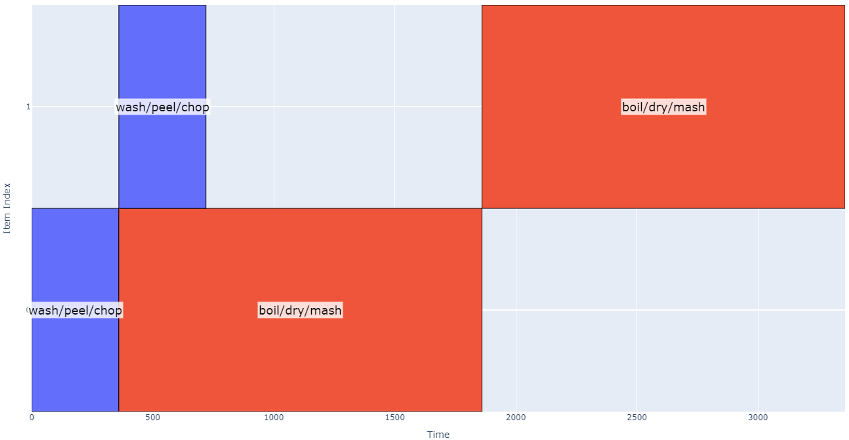
To further extrapolate our example, let’s now assume we are using 16 potatoes to make mashed potatoes. Assuming we still only have two pots to work with, we can only do boiling, drying, and mashing on eight potatoes at a time, which effectively defines two new groups of 8 potatoes and two new summarized operations:

1. Wash/Peel/Chop eight potatoes using 2 pots.

1.1  360 seconds (about 6 minutes) from analyzing previously generated plot.
1.2  Operation conflicts only with itself

1. Boil/Dry/Mash eight potatoes using 2 pots.

2.1  1500 seconds (about 25 minutes)
2.2  Operation conflicts only with itself

Figure 2

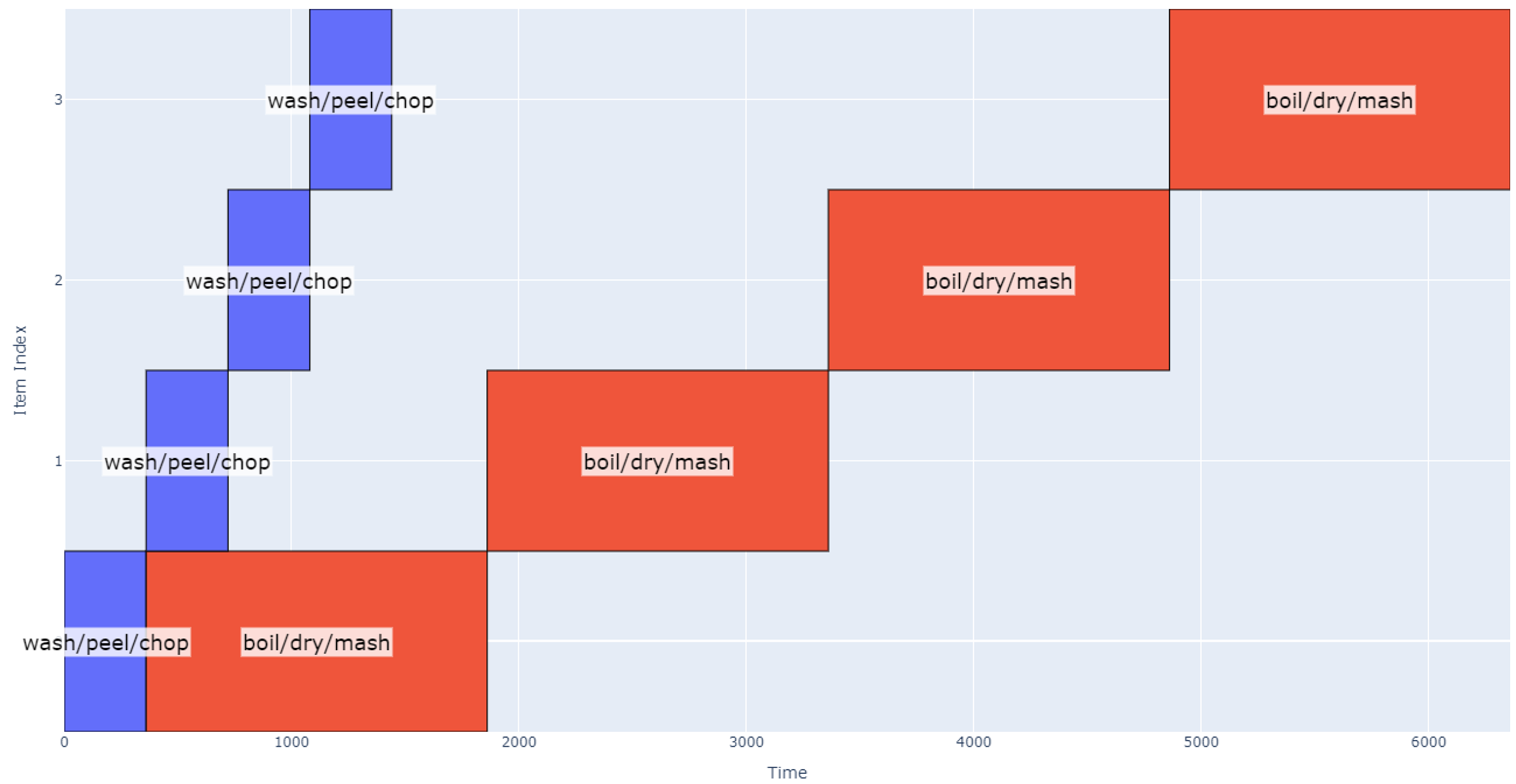
The schedule is now looking at 56 minutes for completion. As the party gets larger and we need to make more potatoes, some other trends are visible.

Figure 3

At this point (four groups of eight potatoes), the schedule gets quite long, and it may make sense to bring in another robot working in parallel, so the total schedule is determined by how long it takes one robot to process two groups of four potatoes.

We will conclude the discussion of making mashed potatoes here as one can begin to imagine the various ways operations, conflicts, and item groups can be represented. Although there are many variables that can be explored in optimizing run time, the goal of this section is to introduce the main concepts of modeling operations using blocks on a graphical schedule, making groups of items to generate a hierarchical schedule, and considering resource conflicts when generating that schedule.

A Python script was developed that implements this scheduling algorithm as described in the example, and it will be included along with this whitepaper.

Schedule Efficiency

One can visually gauge the efficiency of a schedule by observing the amount of white space present in its representation. Using the schedule model discussed above, white space represents time that an item is “waiting” for an operation to be conducted on it. On the other hand, a maximally efficient schedule has operations applied to all items in parallel from start to finish.

One can generate a metric for this efficiency using the following formula.

Note that if we multiply the numerator and denominator by the number of items in the schedule, then we get the ratio between the optimum schedule graph area and the actual schedule graph area; the difference between these two areas is the white space on the actual schedule.

Application Notes

Pitch-Wise Operations

Let’s assume we are designing a robot that makes hot dogs, and there is a need to dispense toppings (ketchup, mustard, and relish) on an incoming stream of hot dogs. For simplicity, assume all hot dogs get the same toppings. As the engineer, we are considering two different designs:

• Concept 1: There is a single nozzle to dispense all three ingredients sequentially on one hot dog at a time.
• Concept 2: The robot has three different nozzles (one for each ingredient), and it can potentially dispense all three toppings at the same time.

There are potential cost savings in using one nozzle, but we would like to explore the improved throughput by using the three-nozzle concept.

Concept 1: Single Nozzle

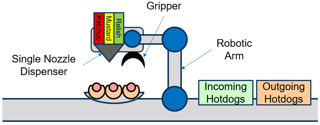
In this case, the system consists of a robotic arm that can pick up one incoming hot dog at a time, place it in a dispense station, move the dispense nozzle, dispense one topping at a time, and deliver a finished hot dog to an outgoing bin. A simplified representation of this robot is represented in the image below.

Figure 4

Our operation sequence is then defined:

1. Fetch and place one hot dog in dispense station: 5 sec.
2. Dispense ketchup: 2 sec.
3. Dispense mustard: 2 sec.
4. Dispense relish: 5 sec (assume this takes slightly longer due to the consistency)
5. Deliver hot dog to outgoing packaging station: 5 sec.

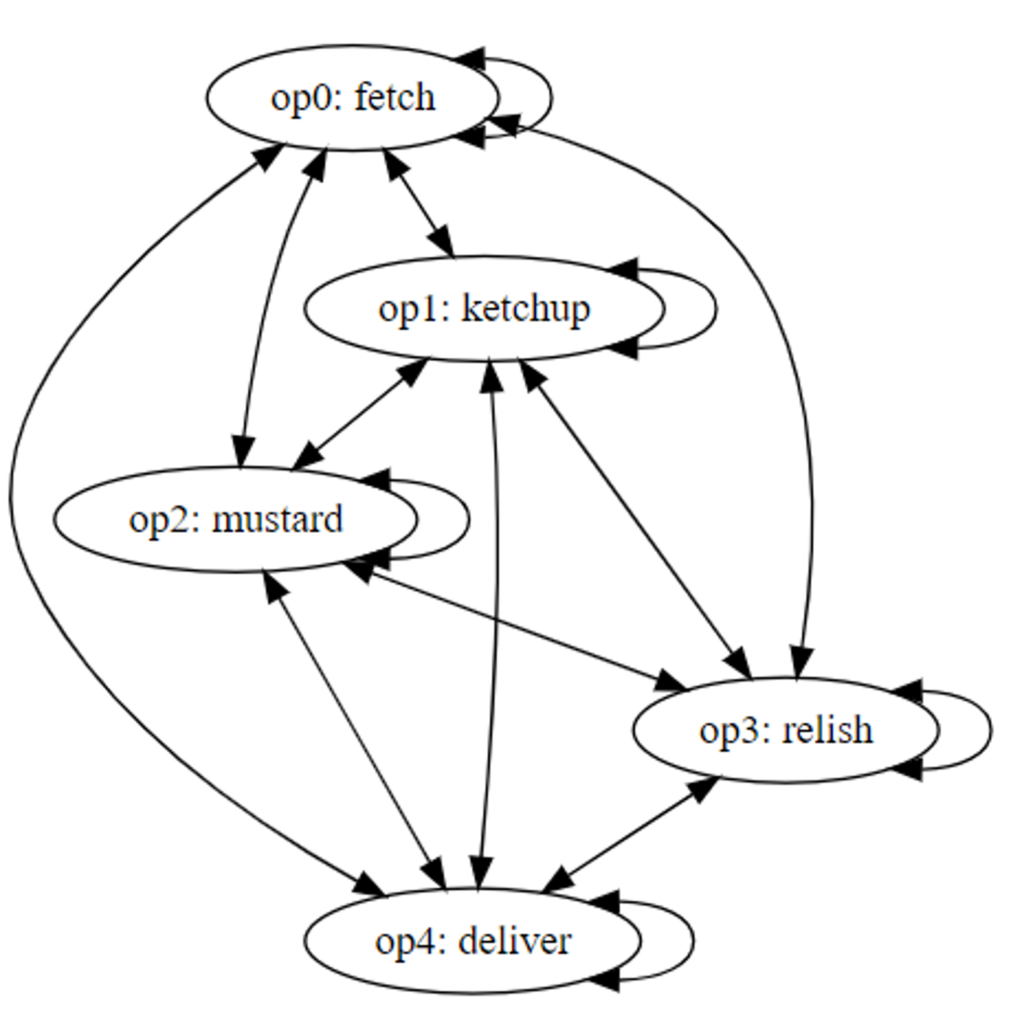
Because there is only one arm, only one operation can occur at a time i.e. resource conflicts exist between all operations.

Figure 5

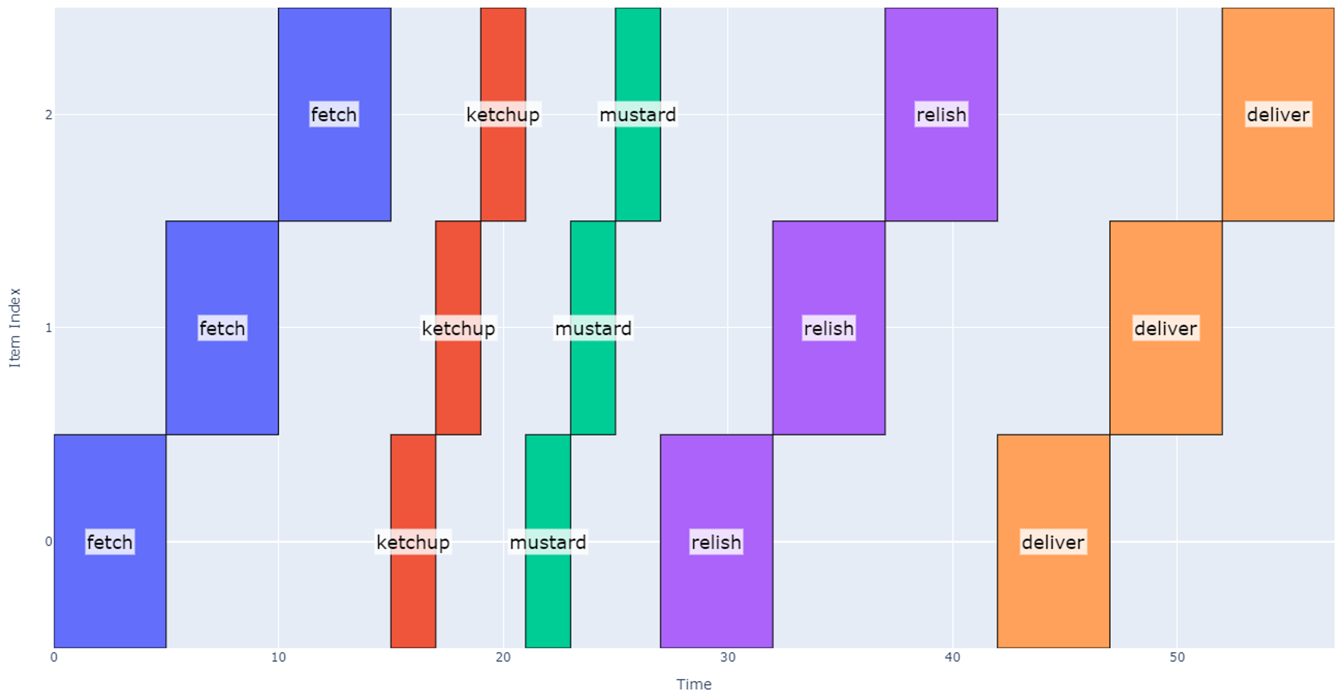
If we are evaluating the schedule duration for three hotdogs as a baseline, the resulting schedule takes 57 seconds.

Figure 6

Concept 2: Three Parallel Nozzles and Pitch-wise Operations

Now let’s explore the case where we can dispense across multiple nozzles at the same time. This effectively removes some resource conflicts so we would expect the schedule to become shorter.

Figure 7

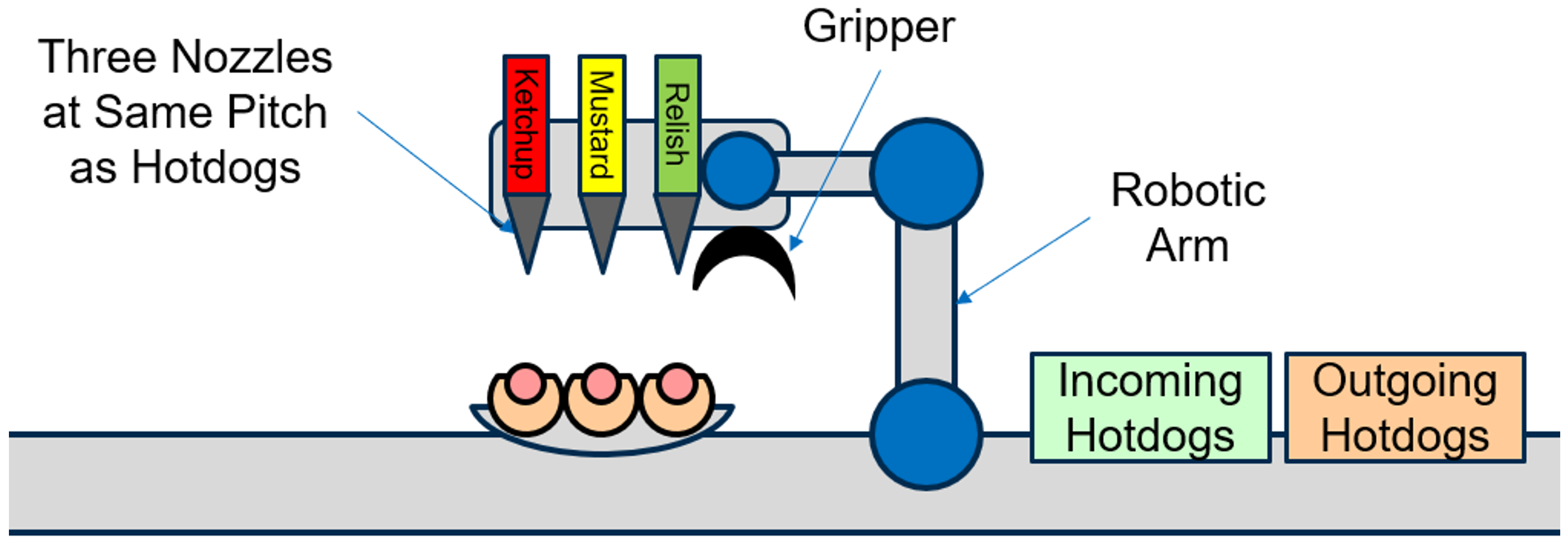
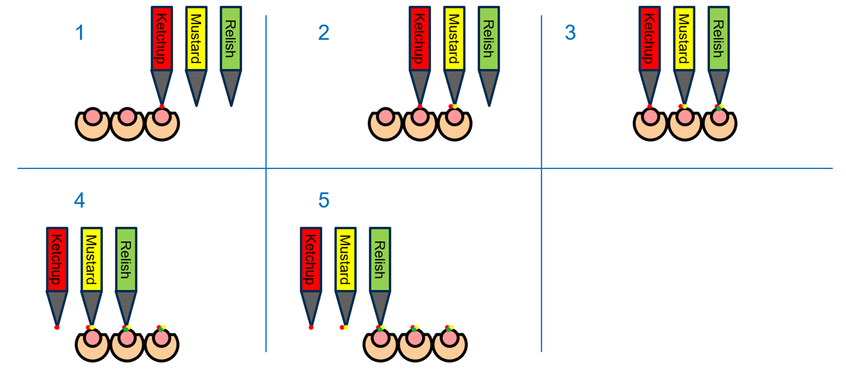
Note that in the above depiction of the system, there are now three independent dispense nozzles, and they have been spaced out to align to three hotdogs (at the same pitch). In this way, dispenses could occur where the arm moves the dispense nozzles horizontally by one hotdog pitch in five stages as shown below:

Figure 8

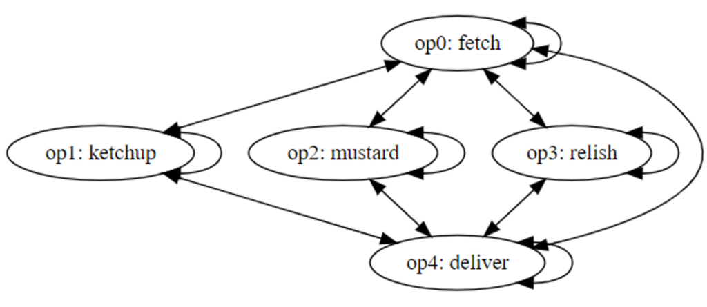
The resource conflict graph now shows that no conflict exists between any of the dispense operations because we can operate each dispense in parallel.

Figure 9

Generating a schedule using the method above results in the model below which suggests it will take 49 seconds.

Figure 10

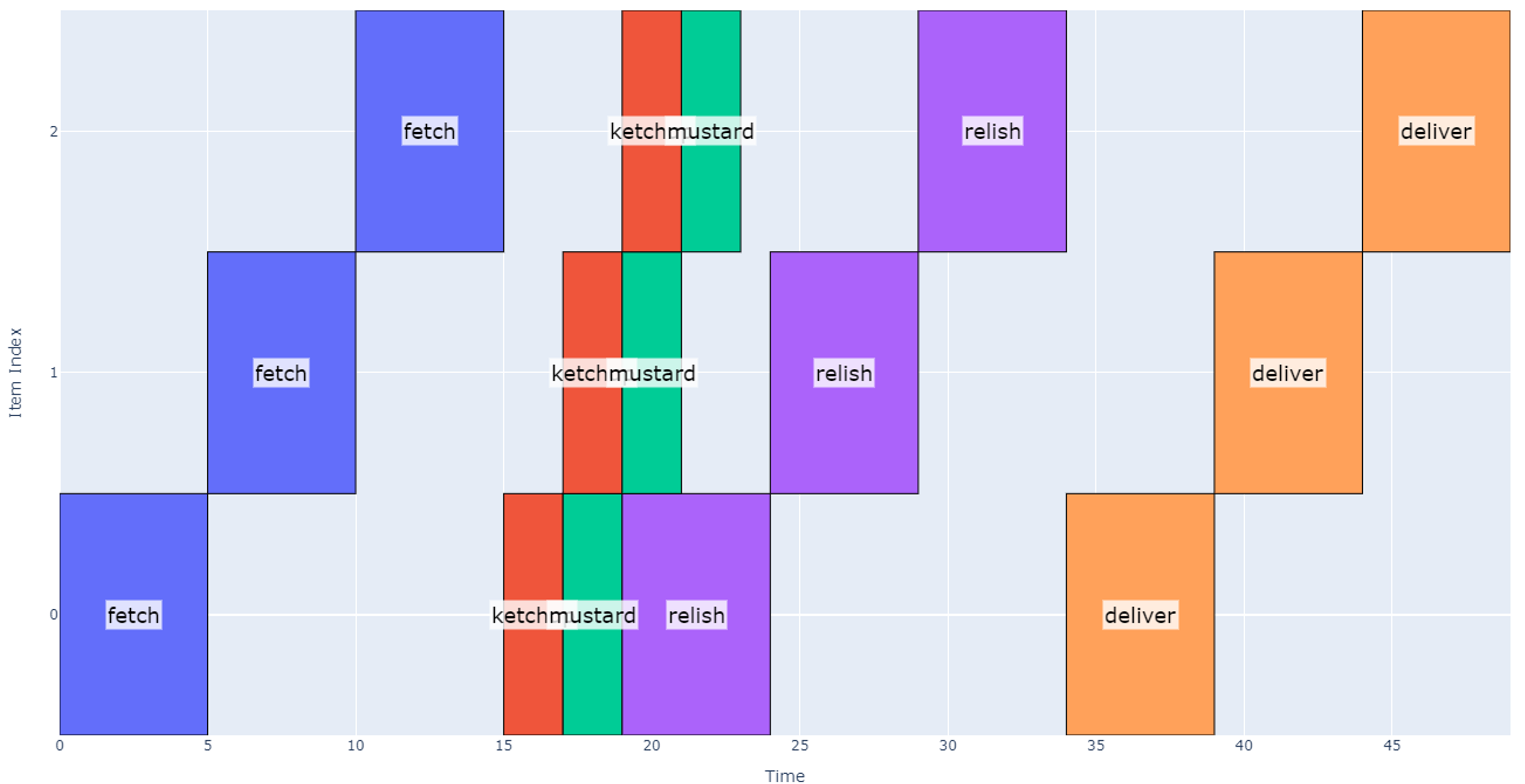
However, note that implementing this schedule is not possible with our current system: while dispensing relish on the first hotdog (between 19 and 24 seconds), the schedule above assumes that mustard can be dispensed on the next two hotdogs sequentially.  Although each topping may be dispensed in parallel, they cannot move independently in our setup (mustard nozzle cannot move relative to relish nozzle).  Therefore, we need to modify our approach to accommodate this reality.

One trivial way to do this would be to allocate the same time for ketchup and mustard dispense as the relish dispense i.e. artificially extend the time it takes to dispense ketchup and mustard.

Figure 11

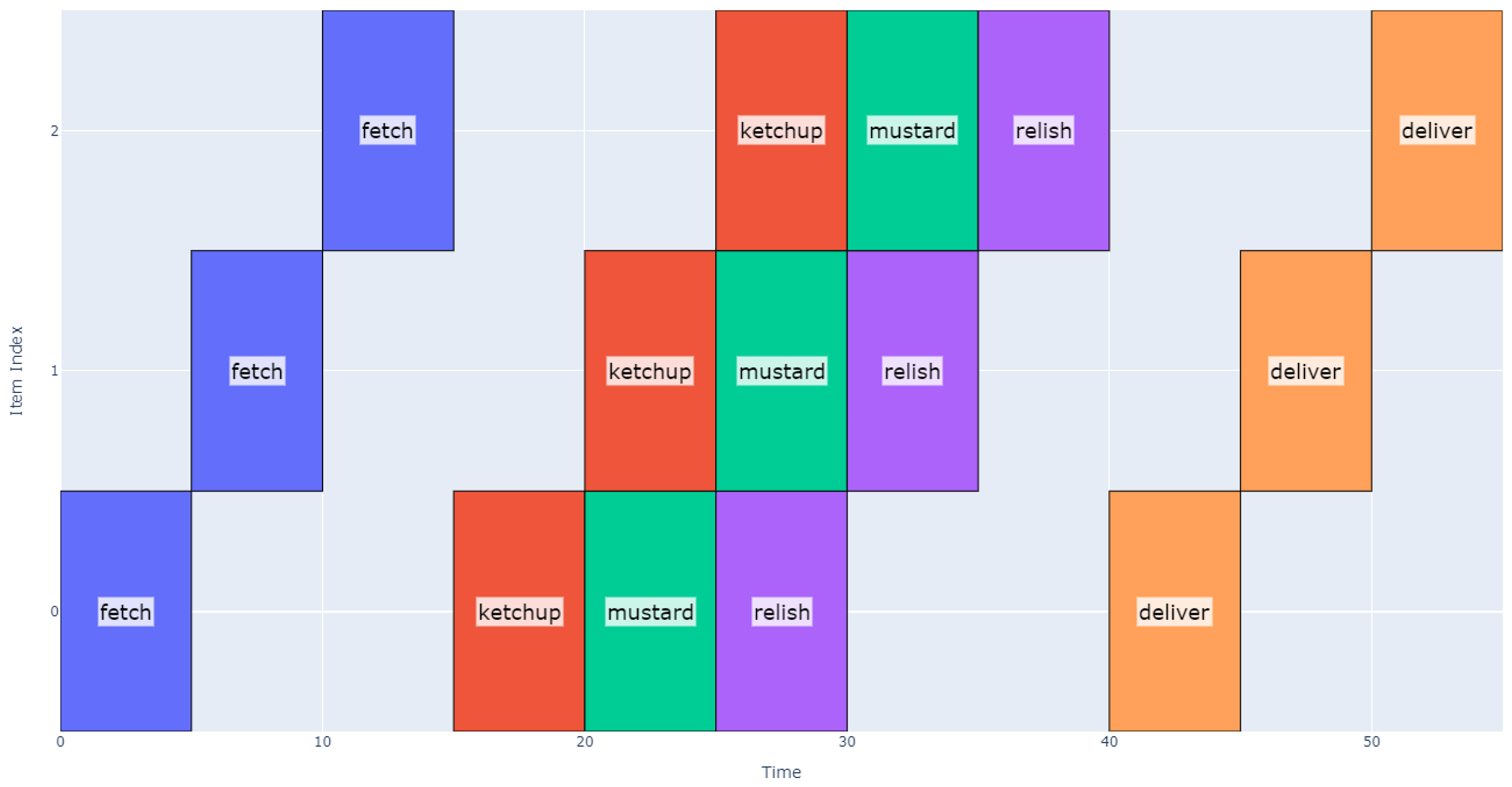
However, this approach yields an unnecessarily long schedule because ketchup and mustard operations do not take as long as relish. When applying this approach to our example, the schedule becomes 55 seconds long, which is nearly as long as Concept 1.  Note that between 15 and 20 seconds we dispense ketchup and then pause for a total of five seconds before moving to the next dispense location, but because it’s the first ketchup dispense, we can move on to the next operations in 2 seconds.

Instead, the best way to model this is by using synchronized start times for each operation: we wait until all operations are finished before starting any new operation. Using this approach, we finally arrive at our more efficient schedule shown below.

Figure 12

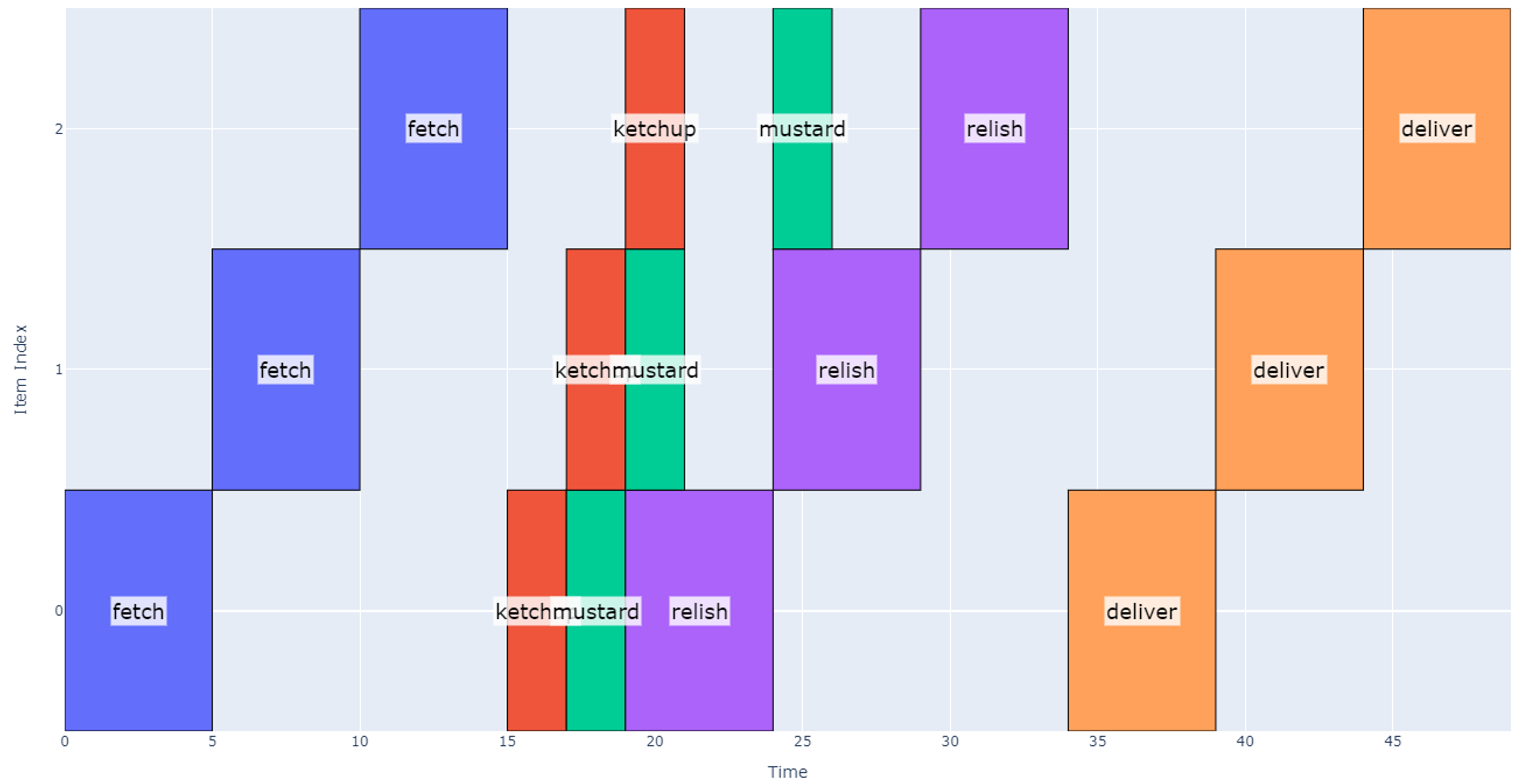
This schedule takes 49 seconds, and we are now able to realize the timing benefit of using multiple nozzles.

Repetitive Schedules with Waiting

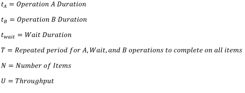
There is another common class of schedules that deserves some attention: schedules that repeat after some amount of waiting. On these schedules, we again have some number of operations that need to be completed, but there is one operation that requires waiting for some minimum time.  During this time, the robot can perform operations on other items, so there is a desire to optimize our efficiency.

Let’s continue with our hot dog example and now imagine we are designing a packaging robot to enclose the hot dogs in a box after toppings have been dispensed.  The packaging robot must:

1. Stage the hot dog box (fold box on stage, place hot dog in box, apply adhesive to box): 20 sec.
2. Wait for adhesive to cure: 3 minutes.
3. Un-stage cured hot dog box: 5 sec.

In this case, note that while we are waiting for the adhesive to cure (a relatively long operation), the robot can stage and prep other hot dogs.  The design challenge then becomes “how many staging slots does the staging area need to maximize throughput”?

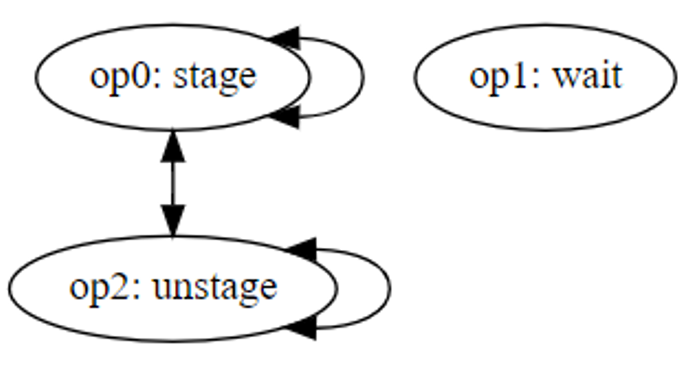
From a resource conflict perspective, wait times are generally represented as an operation with no conflicts.  For simplicity in our example, let’s assume all operations have conflicts with each other except the wait time which has no conflicts.

Figure 13

Numerical Approach

For this design, the items being operated on aren’t individual hot dogs; we will assume that the robot always has an infinite and immediate supply of hot dogs at the input.  Instead, the items of interest are the individual slots where the robot can perform the staging, waiting, and un-staging.  First, assume the staging area has two slots to hold a maximum of two hot dog boxes.  If we were to command the robot to stage, wait, and un-stage hot dogs over and over in these two slots, we would get a schedule like the one shown below.

Figure 14

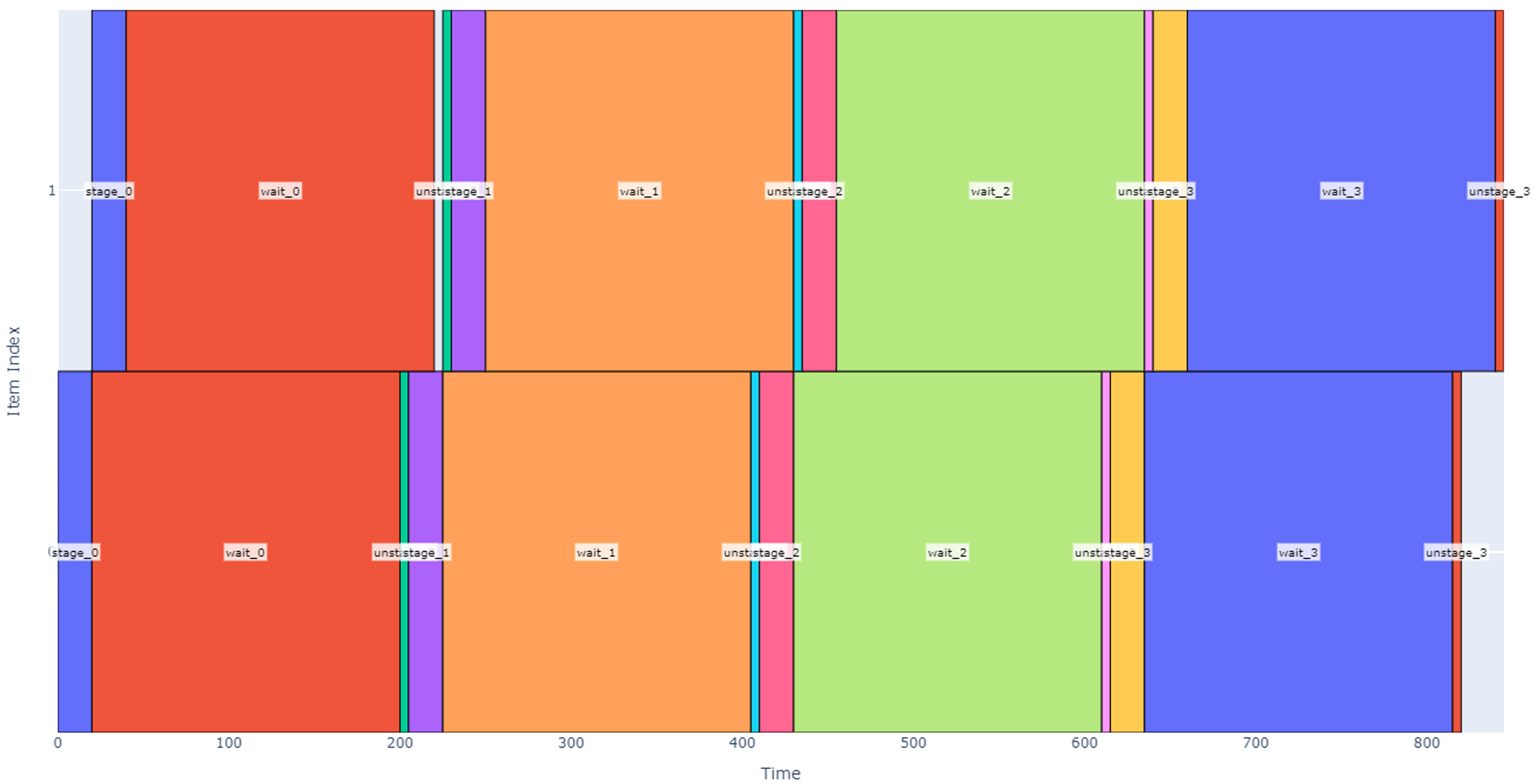
Note that each of the two slots (vertical item axis) stages, waits, and un-stages the hot dog boxes four times in the above depiction.  In the above schedule, four hot dog boxes are prepped in each of two slots over 845 seconds (14 minutes), so our robot throughput is roughly 0.57 hot dogs per minute.

If we wanted to speed this up, one may note that there is a significant amount of time where the robot is waiting for glue to cure and not doing anything (such as the orange boxes overlapping from 250 to 405 sec).  We can utilize the robot more if we enlarge the staging area to four slots.

Figure 15

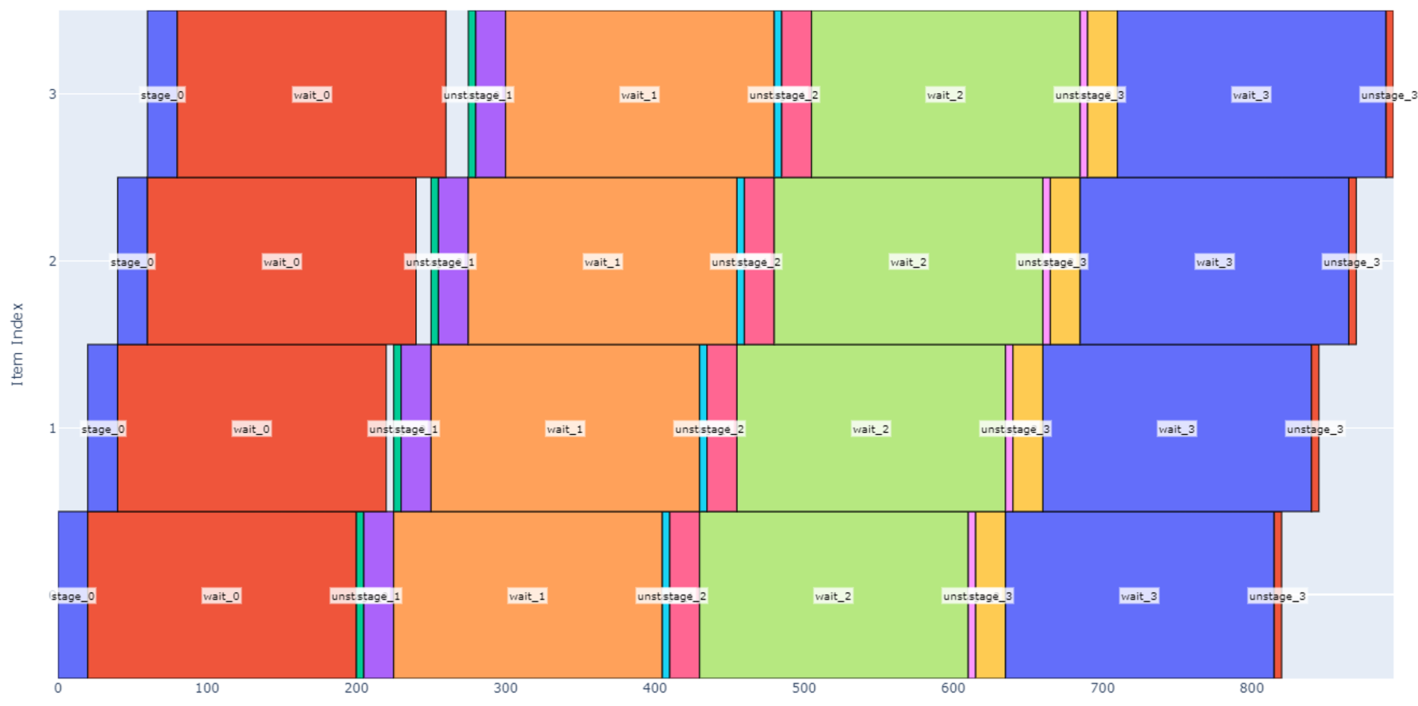
Although our total schedule has lengthened to 895 seconds to process four boxes at each slot, more boxes are processed overall.  With this change, our throughput nearly doubles to 1.07 hot dogs per minute.

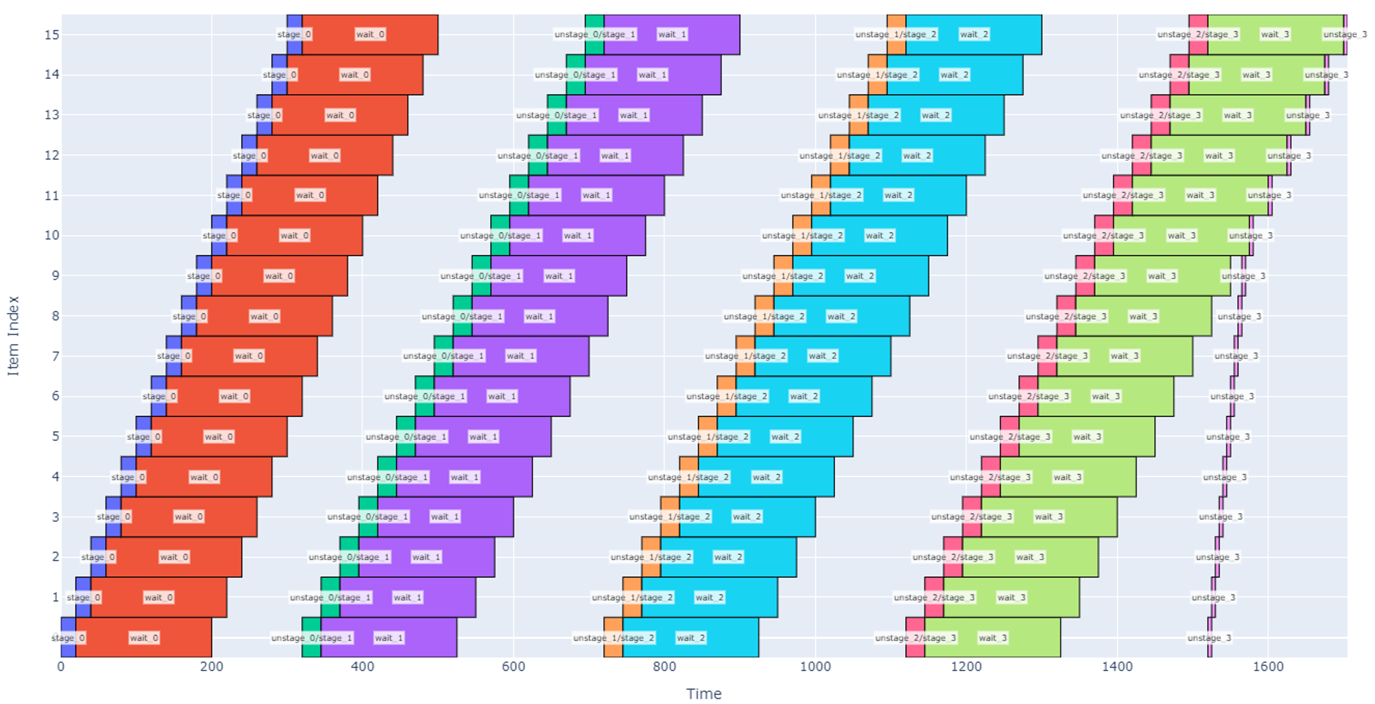
Continuing along this path, however, will eventually lead to a tradeoff: if we have too many slots, the robot will be working very hard to stage and un-stage boxes while some boxes have finished being cured and are waiting to be picked up.  This scenario is shown below with 16 slots.

Figure 16

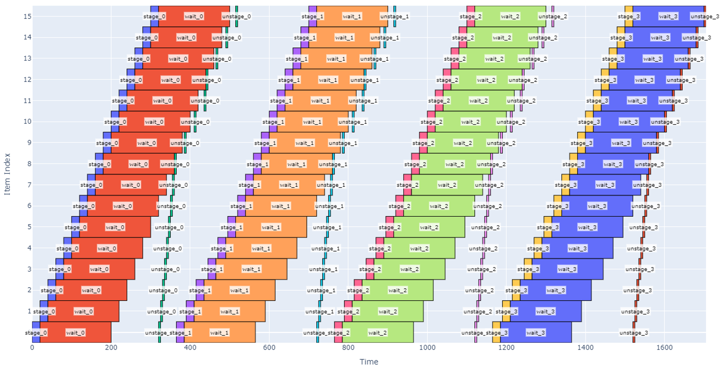
Note that in the schedule above, once the robot finishes staging the box in slot 15, it goes back to slot 0 to un-stage there.  However, there is a lot of white space in the graph indicating that there is significant time where the waiting period is over, and each slot is not having its time fully utilized.

Another notable observation is that the robot jumps around between different non-sequential slots (see the un-stage operations that are isolated from other operations).  This would likely not be desirable so that we can keep the robot motion more predictable and to avoid budgeting extra time for longer moves.  We could either tweak the priority function used by the scheduler or, more simply, change the operations sequence so that un-staging and staging are considered one operation except at the beginning and end of the schedule.

This schedule is easier to implement in practice, and better shows the extra wait time at each slot when there are too many slots.  It is not immediately clear when this tradeoff occurs, so we can numerically evaluate the throughput vs. number of slots.  The graph below solves the schedule for various numbers of slots and determines the throughput and efficiency in each case.  As expected, after around 9 slots are added, there are diminishing benefits from adding more slots.

Analytical Approach

The schedules above have been generated numerically which allows us to estimate the schedule for a specific application with known or assumed durations for each operation.  However, they do not always provide the insight necessary for design decisions: what if we could make un-staging 1-2 seconds faster, would that be more valuable than making the wait time 5 seconds faster?  These types of questions can benefit from an analytical approach for evaluating schedule duration and variable sensitivity.

The example above with a hot dog packaging robot, several packaging slots, and a wait time may be further generalized: let’s redefine the operation sequence to the generic operation sequence below.

1. Operation A
2. Wait
3. Operation B

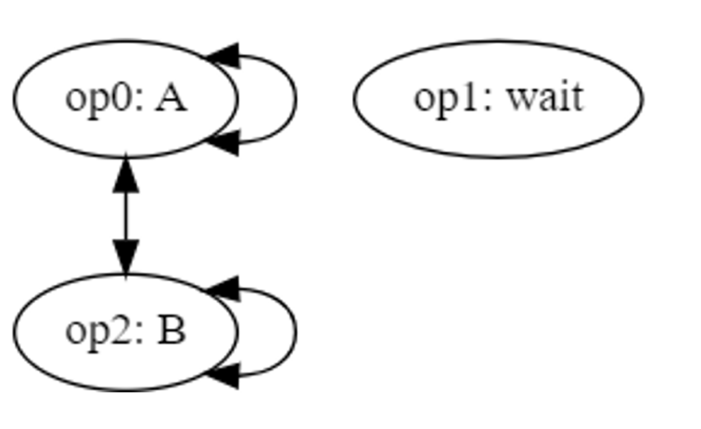
Assume that the system repeats this sequence on each item for some number of cycles.  With conflicts between only A and B, we have the conflict graph below.

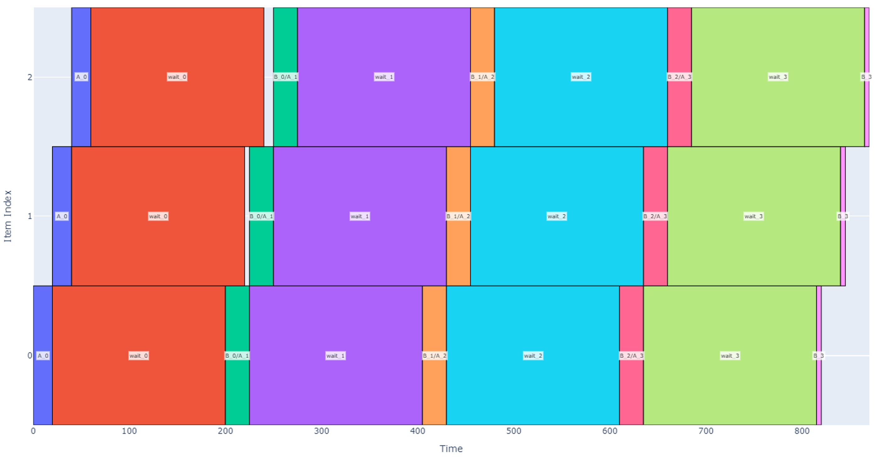
If the operation durations are not known, then there are two different regimes that may occur when scheduling.  In the first regime, the wait time is long relative to the operations and number of items. After each waiting period, the system operates on each item (B then A operations) starting from item 0 then moves on to the next item.  When the B/A operations are complete on the last item, the machine returns to item 0 to wait until it can perform operation B then A again on each item.  We can call this case Regime Alpha and a representative schedule is depicted below with four cycles.

In contrast, if operations A or B get longer or if the total number of items increases, then we enter a new regime, Regime Beta, where the machine is constantly working.  In this regime, as soon as B and A operations are completed on the last item, item 0 has been ready so the machine can jump back to 0 and continue operations.

In this case, we begin to introduce more white space into the schedule (less efficiency) as some items are waiting longer than they need to.

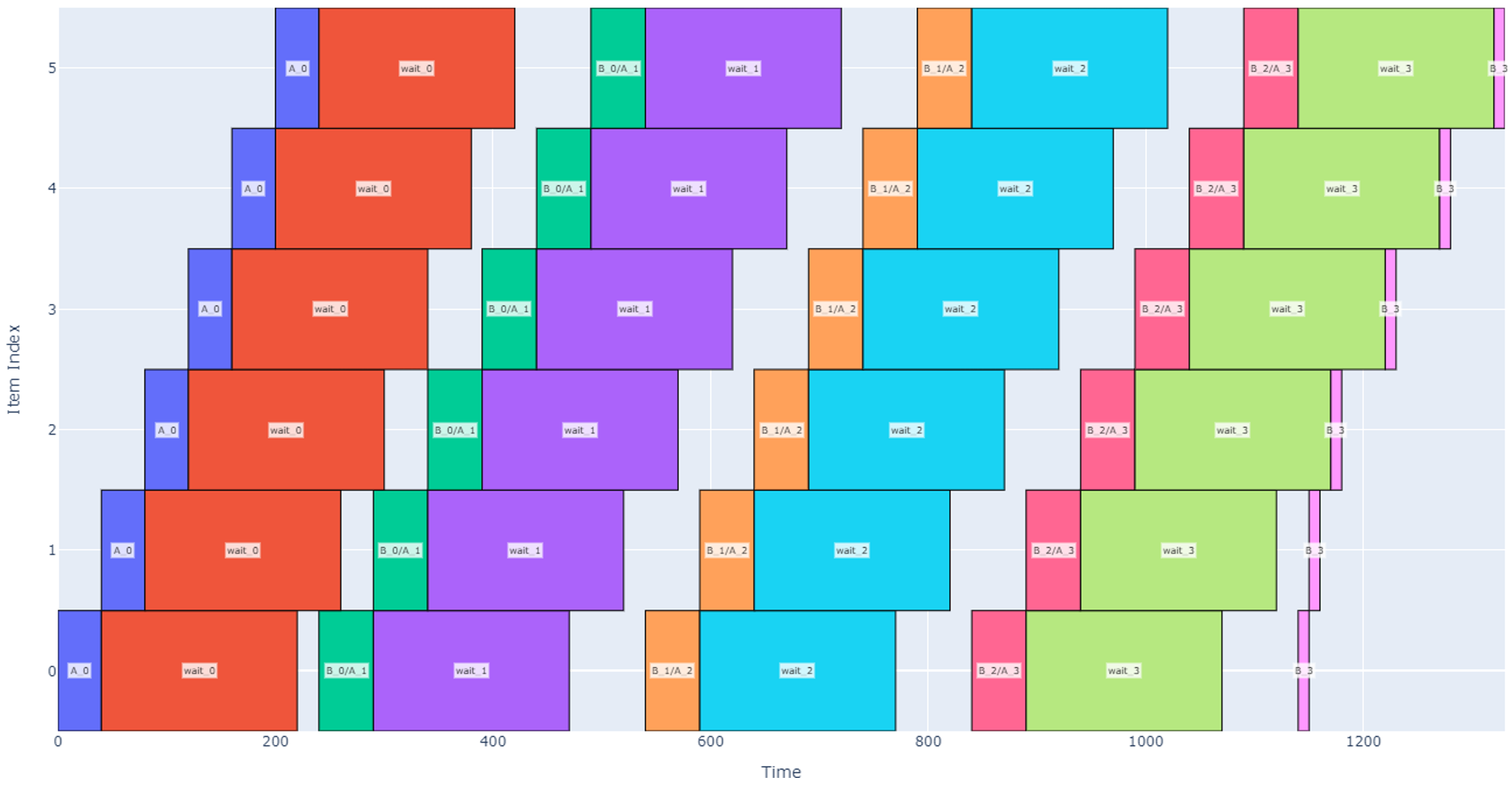
From here on, we will generally be more concerned with the cycles in the middle of the schedule (excluding the first and last cycle) as some unusual patterns emerge there. Instead, the analytical approach is more focused on the long-term pipeline and the behavior over many cycles. Let’s introduce some variables for a cleaner analysis.

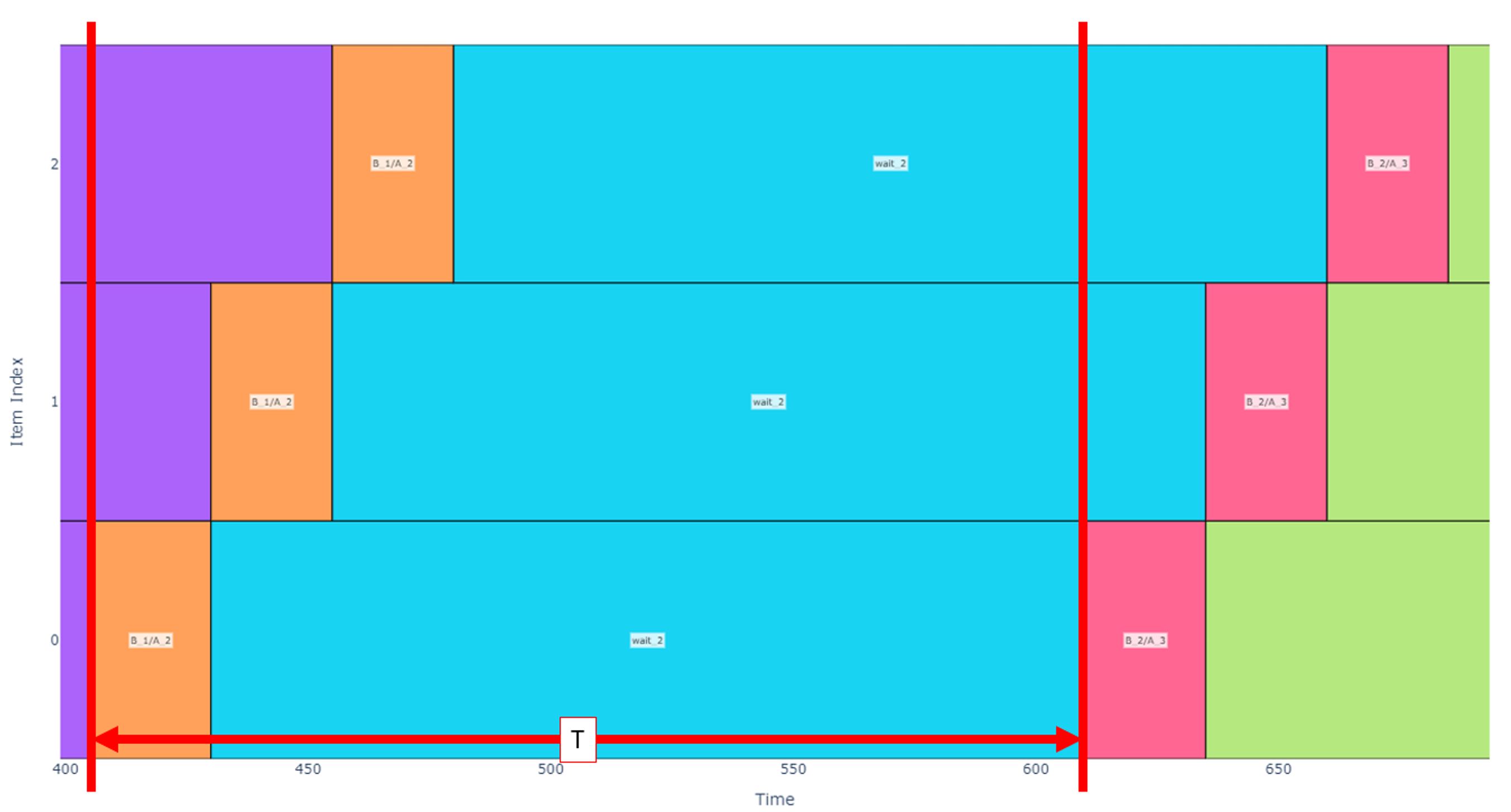
Returning our focus to Regime Alpha, let’s isolate the schedule to just one cycle in the middle of the pipeline.  Below, I have annotated the schedule with red lines to show the start point of when the machine starts operating on item 0, operates on all other items, then returns to begin operating on item 0 again.  This period, T, is our metric of interest because in cases where there are many cycles, the first and last cycle are less important to cycle time, and we can assume that the system throughput scales linearly with this period.  In other words, a shorter T indicates that for a given number of items, there is a greater throughput.

In Regime Alpha, this duration  can be calculated by inspection of the schedule.

The throughput, U, for the system can then be calculated as the number of items to be operated on in a certain time or

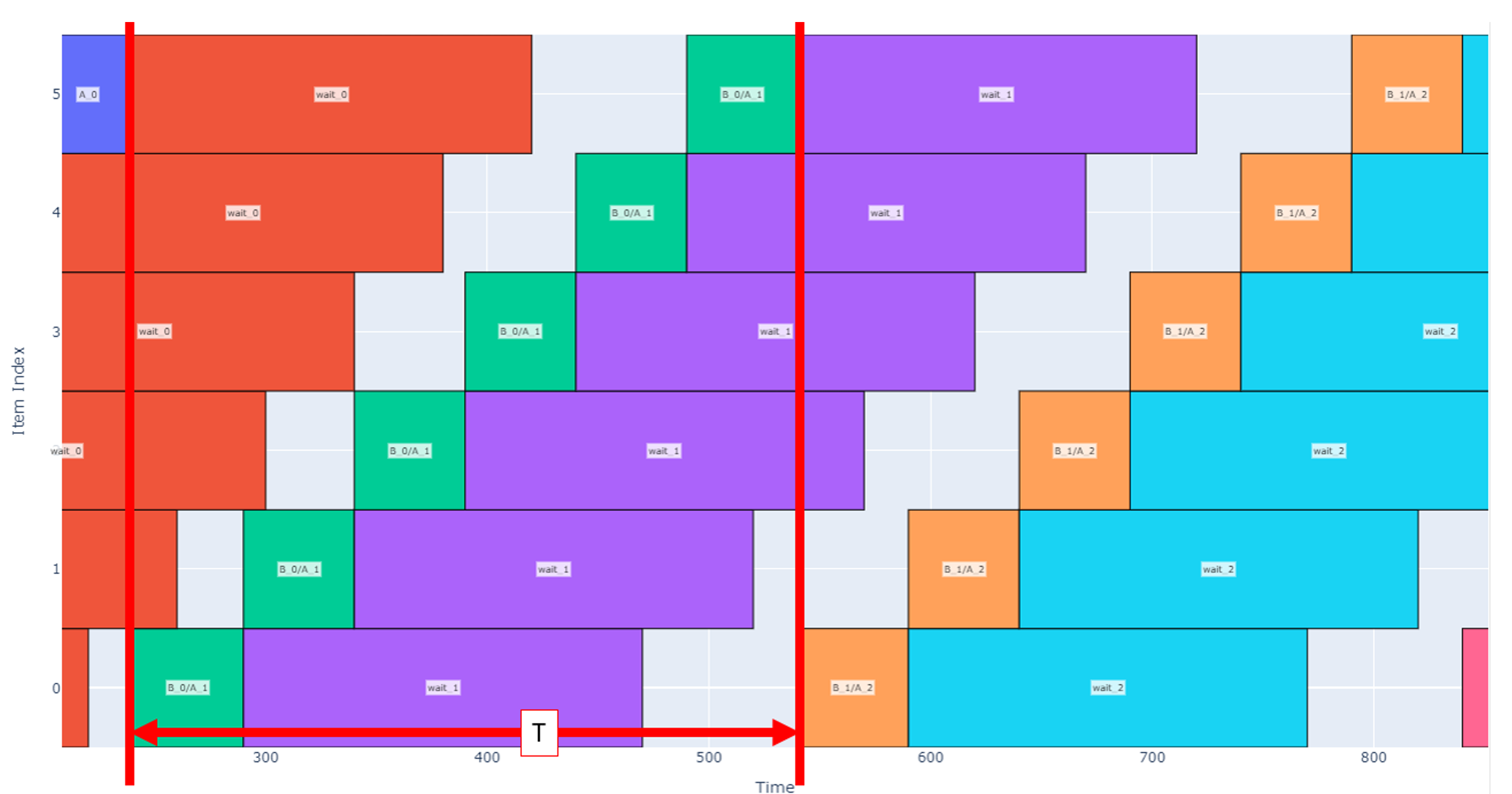
Isolating a schedule in Regime Beta similarly to above, we annotate the period slightly differently.

In this case, the long-term period, T, is agnostic of the wait time and is only dependent on the A and B operation durations and the number of items.  The transition from Regime Alpha to Regime Beta occurs when the time it takes to operate on all items after the first one is greater than the wait time.

Again, we can inspect the schedule to find the period and throughput.

This representation becomes useful in cases where there are tradeoffs between different design parameters.  For example, let’s say we are unsure how long operation A will take, but the number of cycles, number of items, and maximum schedule duration is fixed.  In this case, we want to evaluate the sensitivity of the period, T, to a change in .  Using calculus, we can then get a higher-level interpretation of sensitivity from

Another example that benefits from an analytical approach is to find the maximum number of items before the system transitions from Regime Alpha to Regime Beta (no extra waiting time for each item). From the regime transition equation identified before we can find that

Conclusion

In this paper we have explored some of the various ways that operations can be modeled.  From a basic model and visualization method using blocks on a graph, one can evaluate, analyze, and communicate many scheduling problems in engineering.  This schedule model provides an intuitive means to think through how to best sequence operations, how resource conflicts impact a schedule, and one simple metric for schedule efficiency.

Additionally, various corollaries arise from this model that allow us to better understand schedules in practical applications.  One potential schedule improvement technique is to employ pitch-wise operations that can occur concurrently and have synchronized start times.  After gaining familiarity with a number of schedules, we finally were able to put some of the high-level takeaways into analytical forms that can be used to make better decisions about pipelining problems.  I hope that you will find these techniques useful and that you are able to enhance your ability to tackle scheduling problems in projects to come.

---

Resources 

• Python script for public use